Estimating implicit regularization in deep learning
Information about implicit regularization is embedded in the dynamics of learning. We use gradients of the loss and a proposed regularizer to estimate its unknown parameters.
University of Pennsylvania
We often explicitly regularize models, adding constraints that can improve generalization. We also implicitly regularize through algorithmic and architectural choices, such as early stopping or dropout. Theory can characterize these effects in simplified settings, but complex networks raise the need for empirical estimation and validation.
Our task is to find a mathematically expressible regularizer such that explicitly optimizing the empirical loss augmented by that regularizer mimics an implicitly biased procedure optimizing the loss alone. Given a parametric family of regularizers, we seek to estimate its parameters.
Regularization changes the optimum.
Regularization modifies the objective function, leading to different solutions than strictly minimizing the empirical loss. In this example, an penalty favors smaller weights. At the regularized minimum, its gradient counteracts the nonzero loss gradient.
At the optimum, the slopes cancel.
Gradient matching in multiple dimensions.
A single slope becomes a vector. At the regularized optimum, the loss and penalty gradients point in opposite directions with equal magnitude.
Point & camera controls
Reverse-engineering the regularization.
In Figures 1 and 2, we fixed the regularization and found the weights which minimize the regularized objective function. We can exploit the structure we saw above to reverse-engineer the regularization for a trained model: fix the learned weights and estimate the penalty parameters .
A hypothetical minimum.
We often obtain weights that deviate from the strict loss minimum—for example, because we stop training before the loss has fully converged. Our key assumption is to characterize those learned weights as a minimizer of a hypothetical objective combining the empirical loss and a regularizer . The regularizer need not have been explicitly used during training.
Computing and matching gradients.
For differentiable objectives, stationarity requires the regularizer gradient to cancel the loss gradient. Both derivatives are taken with respect to the model weights and evaluated at the observed weights :
Learning the regularizer. We fit a regularizer model in which the predictive model’s weights are fixed and the regularization parameters are learnable. When exact gradient matching is not possible, we minimize the mean squared error of this matching task. The training data stay fixed, and is the number of weights.
In the next example, the observed weight stays fixed while we estimate the strength of the same quadratic penalty used in Figure 1.
The inverse calculation and its limits
In Figure 3, and with . Their derivatives give the residual . For , minimizing its square has the closed-form solution:
“Estimate ” animates from the current guess to this exact least-squares solution; it is not a simulation of an iterative optimizer.
For , the gradients can cancel exactly. Outside that interval, nonnegative ridge cannot explain the observed weight as an optimum: its best fit leaves a residual. At , every supplies the same zero penalty gradient, so is unidentifiable. A fitted coefficient is an explanation within the chosen family, not evidence that this mechanism generated the weights.
Estimating regularization from training updates
An alternative perspective examines deviations along the training trajectory. At each step, architectural and algorithmic choices can make weight updates deviate from a reference path based on the loss gradient. These deviations provide another set of equations for estimating the regularization parameters, without assuming that the weights are at a minimum.
For the reference update , rearranging gives:
Here and is the step size. We can fit the same coefficient across several updates, or estimate a changing coefficient at each step. Setting recovers the endpoint-matching condition.
The reference must match the question. Comparing ordinary full-batch GD with its own update gives zero discrepancy. To study the effect of finite GD steps, the paper instead compares a discrete step with continuous gradient flow over the same time interval. Figure 5 uses endpoint matching at different iterates; it does not fit these update discrepancies.
Stationarity and identifiability.
These quadratic bowls are convex, so a zero net gradient identifies the minimum. A neural network is more complicated: gradient cancellation alone establishes stationarity, not a global minimum. Several regularizers may explain the same endpoint.
With multiple penalty terms, we fit their coefficients together: . Each weight contributes one equation. If two penalty gradients are nearly parallel, their separate coefficients can be difficult to identify even when their sum fits well.
Recovering an penalty in a neural network.
Before estimating implicit effects, we test whether the method recovers known explicit regularization. Train a small network on noisy samples of a curve. We train with an explicit penalty and withhold its coefficient from the estimator. The estimate uses only the weights and the gradient of the unregularized training loss. During training, this endpoint estimate may be inaccurate because the gradients have not yet reached a balance.
What counts as successful estimation?
We test two distinct claims:
- Recovery of hypothesized regularization. When the regularizer is known or predicted by theory, compare its estimated parameters with the known values.
- Recovery of the original model weights. Replace the training mechanism with the estimated explicit penalty and test whether optimizing the new objective reproduces the learned weights.
The first experiment tests recovery of a known penalty. The early-stopping example tests both claims: reproducing the weights need not uniquely identify the regularizer.
Initialization seed: .
Model, training, and estimator
This is a simplified version of the paper’s explicit elastic-net recovery experiment. Here we estimate one coefficient in a small, single-input network. The paper jointly estimates smoothed and coefficients in a 200-unit ReLU network with 10 inputs, across repeated datasets and penalty settings.
We use mean squared error and , penalizing all parameters, including biases (3 × width + 1 parameters). Full-batch gradient descent runs for up to 20,000 steps. The learning rate is 0.04 × 16 / width (0.04, 0.02, or 0.01) to keep wider networks stable. The data and initialization are reproducible for each seed.
This is a nonnegative least-squares projection of onto . “Gradient explained” is . It is a fit diagnostic, not predictive . Near-zero weights make the coefficient unidentifiable; a near-zero loss gradient makes the explained fraction uninformative. We display a dash for unavailable diagnostics.
For ReLU, we use a zero derivative at a kink. Tanh uses its smooth derivative, . Finite training time and nonsmoothness can leave a residual even when the loss appears stable. This experiment demonstrates explicit-penalty recovery, not proof that an arbitrary implicit bias is ridge regularization.
Estimating the regularization from stopping early.
Theory gives us a concrete example of implicit regularization: for ordinary least squares (OLS), gradient descent with a sufficiently small step size, stopped after a finite number of steps from zero initialization, has the same solution as an explicitly regularized regression. The equivalent penalty is quadratic, , with a closed-form matrix determined by the data, step size, and stopping time. This matrix is the target for gradient matching.
We ask two different questions: can we recover that theoretical matrix, and can an estimated penalty recover the original model weights? A diagonal estimate from one endpoint can recover the weights while differing from theory. A full symmetric estimate uses weights from several independently trained models to recover the matrix. A single ridge coefficient provides a heuristic summary of how regularization decays over training.
The theoretical quadratic penalty and closed-form OLS solution
Let and use the loss . Full-batch gradient descent starts at zero with step size satisfying . At step , its weights minimize , where
The eigenvectors give the penalty’s directions, and its eigenvalues decrease over training. The matrix is generally not diagonal in the original input coordinates. The factor ½ reflects the half-MSE loss convention used here; the paper writes its theoretical penalty with the loss .
For any estimated symmetric matrix , the explicit solution is , provided is positive definite. We solve this system independently to test weight recovery. The estimator receives weights and loss gradients, not the theoretical matrix or its eigenvectors.
Recovering the regularization matrix.
Write the quadratic penalty as . Each square below is an entry , in the original ten input coordinates. Diagonal entries penalize individual weights; off-diagonal entries couple pairs of weights. The theoretical matrix comes from the known early-stopping formula; the estimate comes from matching gradients. With one ridge coefficient, the estimated matrix is .
White in the difference map indicates agreement.
Each point compares one stopped weight with its explicitly regularized solution. The dashed diagonal indicates exact recovery.
Estimation methods and relation to the paper
Absolute matrix error is the Frobenius norm of the difference between the estimated and theoretical matrices. Zero means exact agreement. Gradient matching can be exact even when the matrix is not identified; agreement with theory and recovery of the weights test different claims.
These comparisons correspond to Figure 4 of the paper: full-matrix recovery in panel B, diagonal estimation in panel C, and a scalar ridge summary in panel E. The curvature ratio is the Hessian condition number: the largest curvature divided by the smallest.
We use 160 observations and 10 inputs; the paper uses 1000 observations. We construct X with Hessian eigenvalues ranging from 2 to , use coefficient seed 7 and Gaussian noise with standard deviation 0.3, and run full-batch GD with . Changing rebuilds the design. All endpoints use the same X and the same selected training step; only the true coefficients and noise are resampled.
Diagonal: fit ten signed coefficients in the original input coordinates, . These are not coefficients in the Hessian eigenbasis. A zero weight makes its coefficient unidentifiable. Even with an exact gradient match, a unique minimum requires to be positive definite; the display checks this condition.
Full symmetric: fit all 55 independent entries by minimizing over symmetric matrices. If the system is underdetermined, we select the solution with smallest Frobenius norm. Ten linearly independent endpoints identify the matrix; fewer leave unobserved directions. No theoretical eigenvectors are supplied. The endpoints share a stopping time; the paper also studies estimation across different stopping times.
Scalar ridge: fit , using . The right plot always shows this separate scalar summary, so it has the same meaning under every matrix selection. Its decline need not imply that scalar ridge recovers the full matrix or the stopped weights.
The matrix heatmaps compare against the independent theoretical formula above. Random initialization changes the starting weights for every endpoint while keeping the data fixed; the zero-start theoretical comparison is hidden in that case.
Estimating regularization from neural-network training dynamics.
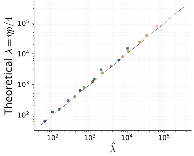
Early stopping characterizes a selected endpoint. We can also estimate regularization from deviations along a training trajectory. Barrett and Dherin predict that, for a smooth loss and sufficiently small steps, discrete gradient descent follows approximately the continuous gradient flow of a modified objective with a penalty on the squared loss-gradient norm:
Here is the step size and is the number of model parameters. In the paper, we estimate this coefficient from the difference between discrete gradient-descent steps and continuous gradient flow, using five-hidden-layer tanh networks trained on MNIST. The estimates closely track the theoretical coefficient across network sizes and step sizes.
How the trajectory comparison is computed
At selected trained checkpoints, we take five full-batch probe steps. For each step, the reference is continuous gradient flow over the same elapsed time, numerically approximated using fourth-order Runge–Kutta integration. The estimator fits the discrepancy using Hessian–gradient products. Comparing a full-batch step with its own linearized loss-gradient update would give zero discrepancy; the continuous-flow reference is essential.
The networks have hidden widths from 50 to 1,600. Checkpoints are selected by validation accuracy among those reaching at least 90% training accuracy. Probe gradients use a fixed subset of 2,048 training examples. The paper gives the full protocol and approximation assumptions.
What the estimates establish.
Gradient matching can recover known explicit penalties and theoretically predicted implicit regularization. Recovering a regularizer’s parameters and reproducing the original model weights are distinct tests: several regularizers may explain the same endpoint.
The paper’s dropout experiments illustrate the limits of a proposed regularizer family. Dropout randomly suppresses hidden units during training. Fitting a scalar ridge penalty reveals variation in the ridge-aligned component across dropout rates and architectures, but explains only a small fraction of the loss gradient. Replacing dropout with that penalty does not reproduce the original test performance.
These experiments provide proof of concept. Extending the approach to larger and more complex systems requires informative candidate regularizers, enough independent gradient equations, and controlled ablations to separate interacting training mechanisms. Even when a candidate captures only part of the effect, its estimate can help characterize how training choices change learning dynamics.
Read the paper on arXiv ↗